This month’s topics:
Learning calculus at 65, in The New Yorker.
New Yorker staff writer Alec Wilkinson takes us along with him on his quest to “penetrate the mysteries of mathematics” (July 8, 2022). As he explains, he was bad in math as a child, and at 65, decided to revisit the subject and to document his experience in a book: A Divine Language: Learning Algebra, Geometry, and Calculus at the Edge of Old Age, published this year by Farrar, Straus and Giroux. In the New Yorker, Wilkinson tells us that he had been turned off by math’s “smugness” and “self-satisfaction” in high school. But he found himself enjoying his exploration anyway. Here are some insights he brought back from the trip. These insights and questions are shared by most mathematicians, and they refute the notion that math is smug and self-satisfied. On the other hand, they are certainly not obvious to someone experiencing mathematics at the introductory level. It is welcome to hear them from a relative outsider, and to read them in a wide-circulation, general-audience medium like the New Yorker.
- Math is unfinished business: even though we have been at it for several thousand years, there are still “many speculations that are not capable of being settled.”
- “Math is both real and not real.” On the one hand, what a mathematician studies exists only in his or her own mind, but on the other mathematicians who have never met agree on the contents of this imaginary world.
- Is mathematics invented or discovered? In particular, the counting numbers: where do they come from? Creation myths usually do not cover numbers, but there they are, and they have their own behavior. “Someone who says that human beings created the operations of arithmetic cannot say that we created the results.” No matter what words or symbols you use for two, plus and four, two plus two will always be four.
Wilkinson’s book was reviewed in the New York Times, July 17: “Math Defeated Him in School. In His 60s, He Went Back for More.”
Hearing shapes, revisited
Rachel Crowell has an article on the Scientific American website (posted June 28, 2022) with the title “Mathematicians Are Trying to ‘Hear’ Shapes—And Reach Higher Dimensions.” This topic was the subject of one of our earliest “Feature Columns,” by Steve Weintraub back in June, 1997: “You Can’t Always Hear the Shape of a Drum.” Crowell’s article covers recent progress on the problem.
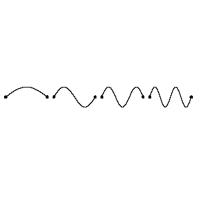
We are all familiar with a big bell sounding a lower note than a small one; similarly, many of us know that long strings vibrate more slowly than short ones. When the frequencies are in the audible range, we hear lower notes from the longer strings. So, all other properties being equal, one can tell by listening if two strings are the same length or not: in that sense, one can hear the length of a string.
Some more about strings. A string fixed at both its ends is limited in the ways it can vibrate. A few of the possibilities are shown in this animation:

Animation here. Note from the animation that modes with shorter wavelength have faster oscillation: in fact, for a string, the frequency of a mode is inversely proportional to its wavelength. Animation from Acoustics and Vibration Animations, website maintained by Dr. Dan Russell, Grad. Prog. Acoustics, Penn State.
Note from the animation that modes with shorter wavelength beat faster: in fact, for a string, the vibration speed of a mode is inversely proportional to its wavelength. As this image suggests, for a string of length $L$ the possible wavelengths are ${2L, L, \frac{2}{3}L, \frac{1}{2}L, \dots}$. So if $\nu$ is the frequency of the first mode, then the set of possible frequencies has to be ${\nu, 2\nu, 3\nu, 4\nu, \dots}$. This ordered list of frequencies is the spectrum of the string.
The head of a drum is the 2-dimensional generalization of a string fixed at both ends. Just as for a string the vibrations of such a membrane are sums of modes, each with its own frequency. For a circular drum, modes and frequencies can be identified explicitly.

The analysis shows that if mode $(0,1)$ has frequency $\nu$, the others have frequencies $1.593\nu$, $2.135\nu$ and $2.295\nu$, respectively (writing just the first three decimal places of each coefficient), and that in mode $(0,2)$ the inner circle’s radius is $0.436$ of the outer’s. Our numbers come from Russell’s Vibrational Modes of a Circular Membrane page, which has animations of these and several other modes.
Crowell’s survey reaches back to a 1966 work by Mark Kac: “Can one hear the shape of a drum?” Kac considers drums that are all cut from the same physical cloth, in that the combination of density, stiffness and tension that determines their mathematical behavior is the same for all of them. He proves for such an ideal drum that its area and perimeter can be “heard” (as above); moreover, he shows that any drum with a spectrum (its set of frequencies of vibration) of the same type as the disc, i.e. ${\nu, 1.593\nu, 2.135\nu, 2.295\nu, \dots }$ has to be circular.
So ideally one can tell by listening if a drum is circular or not. The question remained in general, if two ideal drums are isospectral (same spectrum, so they sound the same), beyond having the same area and perimeter, are they the same shape and size?
As Crowell tells us, it took more than twenty years for this question to be settled. “One Cannot Hear the Shape of a Drum” was published in 1992 by Carolyn Gordon, David Webb and Scott Wolpert. Here is one of the isospectral pairs the team exhibited in their paper.

Recent progress: as Crowell reports, it is now known for triangles and for quadrilaterals with two parallel faces (including parallelograms, rectangles and trapezoids) that sounding the same means having the same shape and size. Crowell goes on to examine isospectral problems in higher dimensions, but leaves us with two unanswered questions in the plane. Are there any convex examples of non-congruent, isospectral pairs? (Note that the Gordon-Webb-Wolpert isospectral pairs are very non-convex). And, quoting from a recent article, “Specifically, it is not yet certain whether the counterexamples [i.e., non-congruent, isospectral pairs] are the rule or the exception. So far, everything points towards the latter.” In other words, differently shaped drums will sound different in general. But this has to be proved.
Gauge theory, for lizards.
Daniel Goldman (Georgia Tech) led a team of four publishing Coordinating tiny limbs and long bodies: Geometric mechanics of lizard terrestrial swimming in PNAS, June 27, 2022. They study the transition from four-footed ambulation in long-legged lizards to pure forward slithering in snakes in a sampling of reptiles with shorter and shorter legs. This work is part of a research direction that started some 45 years ago, and has roots in mathematics (topology and differential geometry) and in theoretical physics.
To recapitulate the history very briefly, it was discovered in the 1970s that two very different fields, topology and theoretical physics, had independently come up with the same concept. Topologists called this concept “connections in principal bundles”, and physicists called it “gauge fields”. The discovery led to important progress in both fields. It is also remarkable that not so long afterwards the same set of ideas turned out to be useful in robotics, in the study of how a mechanism could move forward over terrain or in water by periodically changing its shape (the basic Geometry of self-propulsion at low Reynolds number, by Alfred Shapere and Frank Wilczek, appeared in 1989). The next step was to apply these concepts, known as geometric mechanics, to natural history, in the investigation of how animals crawl and swim, which brings us to lizard terrestial swimming.
In this analysis, the standard use of the term gait to denote the different ways a horse (or other animal) moves forward (e.g., walk, trot, canter, gallop) is generalized to refer to any periodically repeating sequence of postures (in an animal) or configurations (in a robot) that results in locomotion. Mathematically a gait can be studied as a loop in the shape space of an animal or a mechanism.

How does geometric mechanics work? The basic process is easiest to visualize for a simple process like a snake’s slithering across a sandy surface, where the relevant part of shape space is 2-dimensional. It is encapsulated in the next image, taken with permission from an arXiv posting by Jennifer Rieser (also at Georgia Tech) and ten collaborators.

Roughly speaking, if the creature has taken a particular shape $s$, and starts to wiggle its body in a certain way, that will make it start to move in a certain direction. This change in position can be drawn as a vector in the copy of position space associated to the initial shape $s$. Now the creature has a new shape $s’$; it wiggles again, and produces a new change in position: a vector in the copy of position space associated to $s’$. As the creature continues to execute its gait, it will eventually return to its original position $s$. When these infinitesimal vectors are summed up around the closed loop (blue) corresponding to the gait, the integral gives the displacement resulting from one cycle.
Goldman and his team start from the observation that, just as Rieser et al. had observed for pure slithering, the periodic changes in reptilian body shape during locomotion can be approximated by a cycle of combinations of two modes, like the first two of the string analyzed above: one where the body oscillates between ( and ), to use a graphical shorthand, and one where it oscillates between S and Z. Their shape space is consequently very much like Rieser’s, but with fore and hind limbs also taken into account.
They report: “… we find that body undulation in lizards with short limbs is a linear combination of a standing wave and a traveling wave and that the ratio of the amplitudes of these two components is inversely related to the degree of limb reduction and body elongation.” This surprisingly mathematical statement implies that for a long-legged lizard, the loop in shape space corresponding to its gait collapses to a straight-line path going back and forth from ( to ); whereas for a limbless snake, the gait mixes the ( ) mode with the S Z mode in such a way as to produce a traveling wave moving down the creature’s body and making it progress forward.


For more background I recommend Geometric Phase and Dimensionality Reduction in Living (and Non-living) Locomoting Systems, a lecture given by Daniel Goldman in Trieste in 2019. It gives details about how the connection form—the mathematical name for the process illustrated in Rieser et al.‘s diagram—can be derived experimentally in each case. Towards the end of the lecture Goldman explains how a “height function” defined on shape space can be calculated for such a connection. This is the same computation that yields the Gaussian curvature in Riemannian geometry, and it allows optimal gaits to be designed for robots by choosing paths that enclose the largest amount of what would be positive curvature.
The link between connections and gauge theory has an elementary presentation in Fiber Bundles and Quantum Theory, an article Herb Bernstein and I wrote for Scientific American in July, 1981. Some historical details can be gleaned, among other topics, from a 2008 video interview of C. N. Yang and Jim Simons.