
One of the fundamental forces in the universe is the weak force. The weak force is involved in holding atoms together or breaking them apart...
Putting a period on mathematical physics
Ursula Whitcher
Mathematical Reviews (AMS)
You've heard of periods at the ends of sentences and periods of sine waves. The word period also has a special meaning in number theory. These periods are surprisingly useful for solving problems in particle physics. In this month's column, I'll tell you more about what periods are, where the physics comes in, and how all of this relates to the geometry of doughnuts.
From doughnuts to integrals
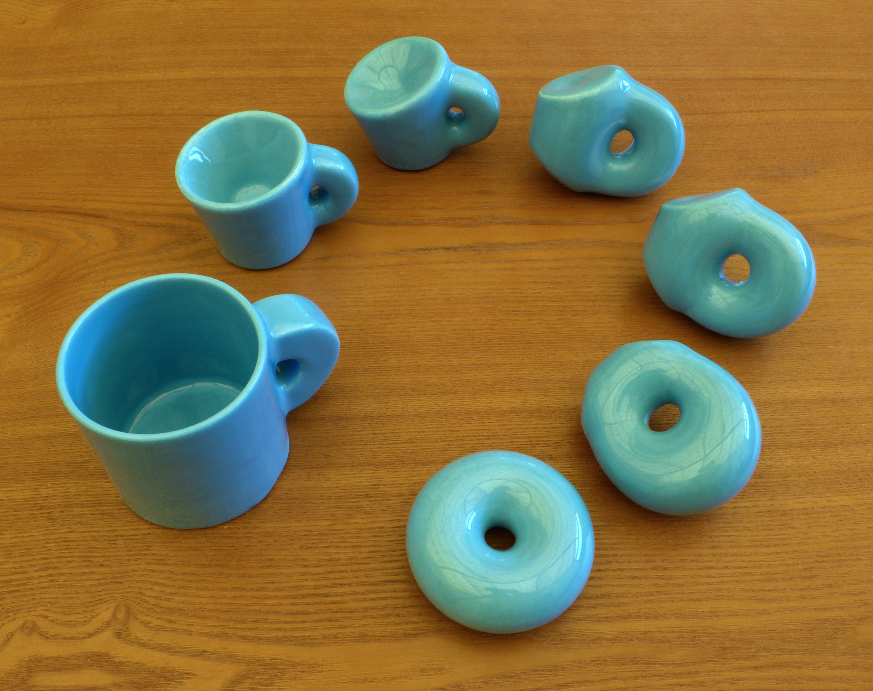
Maybe you've heard the joke that a topologist can't tell the difference between a coffee cup and a doughnut. (If it's new to you, check out a beautiful illustration of the transformation by Keenan Crane and Henry Segerman.) Geometers are able to distinguish coffee cups from doughnuts. We can even tell the difference between types of doughnuts. For example, here's a fat, cakey doughnut:

Here's a skinny, crunchy doughnut:

But the geometry of doughnuts is so fascinating that, once you begin examining it, it's hard to think about anything else!
Let's describe the difference between our two doughnuts more formally. An idealized mathematical doughnut surface is called a torus. We can characterize the shape of a torus using two circles, one that goes around the outside and one that goes through the hole in the center. On a fat, cakey torus, these two circles are roughly the same size.

On a skinny, crunchy torus, the outer circle is much larger than the inner circle.

In these examples, the circles are easy to measure. But sometimes tori appear in more complicated ways. For example, suppose $x$ and $y$ are complex variables and $t$ is a complex parameter. Consider the solutions to the equation
\[y^2 = x(x-1)(x-t).\]
This is the famous (for number theorists) Legendre family of elliptic curves. If we throw in a solution "at infinity," then, topologically speaking, it is a family of tori. It's hard to graph the solution to an equation in two complex variables, but we can graph the real values. Here's what it looks like when the parameter $t$ is set to be equal to 3:

You can think of graphing the real points as slicing through the doughnut at an angle. In this graph, you see a skewed version of one of the circles and part of a second circle.
Measuring the lengths of these two circles is tricky. There is a general mathematical strategy from calculus class that we can try: set up an integral to measure the arclength. In this case, the appropriate integral turns out to be:
\[\int_\gamma \frac{dx}{y} = \int_\gamma \frac{dx}{\sqrt{x(x-1)(x-t)}} \]
Here, the integral is over an appropriate simple closed curve $\gamma$ in the torus/elliptic curve.
But there's a problem! I'll let a cartoon of an easily confused orange cat explain it.

The cat isn't lying: this integral is really hard. Standard techniques from calculus class do not work. In fact, this integral has no closed-form algebraic solution.
Periods and differential equations
The integral $\int_\gamma \frac{dx}{\sqrt{x(x-1)(x-t)}}$ is an example of a period. For a number theorist, a period is a number that you get by finding the integral of an algebraic expression over an appropriate subspace. (Technically speaking, we should be able to describe the regions we are integrating over using inequalities and systems of algebraic equations whose coefficients are rational numbers.)
Many interesting constants, such as $\pi$ and $\log 2$, can be written as periods. There are huge and interesting questions about periods: for example, how can we characterize which numbers arise as periods? Using operations on integrals, one can show that adding or multiplying periods produces a new period. This gives periods the structure of a ring. Another big open question is describing all the relations that the ring of periods satisfies.
Let's get back to trying to understand our specific period, $\int_\gamma \frac{dx}{\sqrt{x(x-1)(x-t)}}$. We know that the result of the integral is a number that depends on the parameter $t$, so let's think of the integral as a function $P(t)$. We can take derivatives of $P(t)$:
$$\frac{d}{dt} \int_\gamma \frac{dx}{\sqrt{x(x-1)(x-t)}} = \int_\gamma \frac{d}{dt} \frac{dx}{\sqrt{x(x-1)(x-t)}}.$$
As we take derivatives, the expression under the integral sign becomes more complicated, but it keeps the same general shape. By finding a common denominator, we can identify a relationship between $P(t)$, $P'(t)$, and $P''(t)$:
\[ t(t-1) P''(t) + (2t-1) P'(t) + \frac{1}{4} P(t) = 0.\]
This is a differential equation! (It's called the Picard-Fuchs equation, after the French mathematician Émile Picard and the German Jewish mathematician Lazarus Fuchs.) As a second-order differential equation, this Picard-Fuchs equation has two independent solutions. These solutions correspond to the two different circles on the torus.
A standard method for solving differential equations is to use an infinite series. In this case, one of the solutions to the differential equation for our period can be written in terms of the following series:
\[\sum_{n=1}^{\infty} \frac{((\frac{1}{2})(\frac{1}{2} + 1)\cdots (\frac{1}{2} +n-1 ))^2}{(n!)^2}t^n.\]
The numerator involves an expression, $(\frac{1}{2})(\frac{1}{2} + 1)\cdots (\frac{1}{2} +n-1 )$, that looks rather like a rising factorial shifted by $\frac{1}{2}$. If we replace this expression by the shorthand $(\textstyle{\frac{1}{2}})_n$, we get a more compact notation for our series:
\[\sum_{n=1}^{\infty} \frac{(\textstyle{\frac{1}{2}})_n^2}{(n!)^2}t^n.\]
This is a famous series known as the hypergeometric series, with numerator parameters $\frac{1}{2}, \frac{1}{2}$ and denominator parameter 1 (since there's only a single factorial in the denominator). The whole series is sometimes expressed by the even more compact notation ${}_2F_1\left(\textstyle{\frac{1}{2}, \frac{1}{2}}; 1 \,|\, t \right)$.
For more details about the solution process, including a description of the second independent period, see Don Zagier's in-depth essay The arithmetic and topology of differential equations. I'd like to show you a more complicated period that shows up in theoretical physics.
Sunsets and Feynman diagrams
In particle physics, describing the interactions between fundamental particles such as electrons and photons involves doing difficult integrals. (Even worse, from a mathematician's standpoint, these integrals may not always be well-defined!) Physicists organize these computations using diagrams called Feynman diagrams of increasing complexity. There are specific rules for creating and manipulating Feynman diagrams, but at a first approximation, one can imagine they tell stories about particles that meet, interact and perhaps undergo a transformation, then go their separate ways.

One of the fundamental forces in the universe is the weak force. The weak force is involved in holding atoms together or breaking them apart. It's the force that controls the process of radioactive decay and makes carbon-14 dating possible.

One can calibrate carbon-14 dating using tree rings. Photo by Bill Kasman (public domain).
To do computations involving the weak force, one must work with Feynman diagrams that contain loops. Here's a Feynman diagram with two loops that is sometimes called the sunset diagram.

The American mathematician Spencer Bloch and the French physicist Pierre Vanhove teamed up to study the sunset diagram. To simplify the problem, they worked with a model where there are only 2 space-time dimensions. (Imagine particles moving back and forth along a line as time passes.) They assumed that all the particles generated during the interaction have equal mass $m$, that there's a fixed external momentum $K$, and they threw in a constant $\mu$ to balance the units. The result is the following sunset integral:
\[\mathcal{I}_\circleddash = \frac{\pi^2 \mu^2}{m^2} \int_0^\infty \int_0^\infty
\frac{dx\,dy}{(1+x+y)(x+y+xy) - xy \frac{K^2}{m^2}} \]
This integral is really, really hard!
One of the key problems is that the denominator, $(1+x+y)(x+y+xy) - xy \frac{K^2}{m^2}$, might be 0. To understand more about where the denominator vanishes, we can set $t=\frac{K^2}{m^2}$. The result is a family of curves that depends on the parameter $t$:
$$(1+x+y)(x+y+xy) - t xy =0.$$
Here's the resulting graph for $t=11$.

The features of this graph might look familiar. We've got a skewed circle and part of another circle—the doughnut slices are back! In other words, $(1+x+y)(x+y+xy) - t xy =0$ is a parametrized family of elliptic curves.
Bloch and Vanhove pursued a strategy that might seem familiar. They set $\mathcal{J}_\circleddash = \frac{m^2}{\pi^2 \mu^2} \mathcal{I}_\circleddash$ to simplify the units, then looked for a differential equation involving $\mathcal{J}$:
\[\frac{d}{dt} \left(t(t - 1)(t - 9) \frac{d}{dt} \mathcal{J}_\circleddash \right) + (t-3) \mathcal{J}_\circleddash = -6.\]
Because the right-hand side of this differential equation is not zero, solving it is more complicated than solving the differential equation we saw earlier. Standard differential equation methods approach this kind of problem in two steps. First, solve the homogeneous equation where we pretend the right-hand side is zero. Then, find a solution to our inhomogeneous equation where the right-hand side is a nonzero constant.
Bloch and Vanhove showed that the homogeneous solutions to the Picard-Fuchs differential equation for $\mathcal{J}_\circleddash$ can be written in terms of the classical hypergeometric series ${}_2F_1\left(\textstyle{\frac{1}{12}, \frac{5}{12}}; 1 \,|\, - \right)$. This series places rising factorials involving $\frac{1}{12}$ and $\frac{5}{12}$ in place of the $\frac{1}{2}$ we saw earlier. I've used $-$ to indicate that a more complicated expression is plugged in for the series variable.
To solve the full inhomogeneous equation, we need another special constant, $\mathrm{Li}_2(z)$, known as the dilogarithm. The dilogarithm can be written as an infinite series. When $|z|<1$,
\[\mathrm{Li}_2(z) = \sum_{k=1}^\infty \frac{z^k}{k^2}.\]
The dilogarithm is also a period! We can write it using a double integral.
\[\mathrm{Li}_2(z) = \iint_{0 \leq u \leq v \leq z} \frac{du\,dv}{(1-u)v}.\]
Thus, periods give us a precise way to describe the solutions to the sunset diagram integral—as well as a reason to eat doughnuts!
Further reading
- Spencer Bloch and Pierre Vanhove, The elliptic dilogarithm for the sunset graph. J. Number Theory 148 (2015), 328–364. MR3283183, arXiv:1309.5865 [hep-th].
- Maxim Kontsevich and Don Zagier, Periods. Mathematics unlimited—2001 and beyond, 771–808, Springer, Berlin, 2001. MR1852188, IHEP.
- Stefan Müller-Stach, What is... a period? Notices of the AMS, September 2014.
- Don Zagier, The arithmetic and topology of differential equations. European Congress of Mathematics, 717–776, Eur. Math. Soc., Zürich, 2018. MR3890449, MPIM.
- Don Zagier, The remarkable dilogarithm. J. Math. Phys. Sci. 22 (1988), no. 1, 131–145. MR940391, MPIM.
Acknowledgments
I thank the Isaac Newton Institute for Mathematical Sciences, Cambridge, England for support and hospitality during the K-theory, algebraic cycles and motivic homotopy theory program, where I presented a version of this material during the institute's 30th birthday celebrations. This
work was supported by EPSRC grant no EP/R014604/1.